Modeling System Resource Usage for Predictive Scheduling

*Note: Full Github repo with code available here.*

This post has also been featured on Manifold's blog.

As an Insight Data Science Fellow, I consulted with Manifold for a project using machine learning and neural networks to model and predict network usage. Manifold is a company that offers startups and new developers a simple yet revolutionary platform to manage their applications and cloud resources in one place. Manifold also serves as a marketplace for additional applications and services, as well as an easy way to work with multiple APIs in one location.

As a consultant, I wanted to get a sense of Manifold’s needs to help them reach their goals. Manifold was interested in gaining a sense of their current network resource usage and provisioning. In addition, Manifold wanted to move towards a machine learning approach to to make real-time predictions and automate scheduling of provisions. This was an exciting new challenge.

The Challenge

Historically, companies like Manifold have to balance the competing needs of minimizing cost of paying for CPU bandwidth, for example, but also minimizing downtime by over-provisioning. This was even evidenced in the publicly available dataset from the TUDelft archive I used for my analysis. This data had similar characteristics to Manifold’s actual data.

Therefore, my role as a consultant was to develop a model that will provide a more intelligent prediction of resource usage.

Here is how I translated Manifold’s business objectives into an actionable deliverable:

First, I used time-series analysis, advanced regression techniques, and time series cross-validation in Python (using scikit-learn) to characterize resource usage as well as identify important predictive features.

Next, I implemented DeepAR, a recently developed built-in algorithm from Amazon Sagemaker (hosted on AWS) to help Manifold shift towards real-time analytics. Amazon SageMaker DeepAR is a supervised learning algorithm used to forecast time series using recurrent neural networks (RNN). Below is a summary of what I did for Manifold.

Blog Outline

Part 1. Characterizing Manifold’s Resource Activity (Python, scikit-learn)

Part 2. Real-Time Pipeline (AWS, Recurrent Neural Network) Part 3. Actionable Deliverables

Part 1. Characterizing Manifold’s Resource Usage

Step 1: Develop Preprocessing Pipeline

I started by pulling the activity traces from 500 Virtual Machines (VMs) over a three-month time period into a pandas data frame using an EC2 instance on AWS (using Python). I first wanted to get a sense of network usage on a larger scale. To do so, I converted the timestamp, which was in Unix epochs to a pandas date-time index. Then, I filled in the occasional missing value using the ‘ffill’ function from pandas, which is a forward propagating function that fills in a missing value with the last observed value. I wanted a broad view of the data, so I aggregated (i.e., summed) CPU usage across all 500 VMs on a coarser time granularity (hourly). Next, I engineered the following 5 new features for Manifold: time lags, hour of day, day of the week, number of cores in use, and the difference in CPU usage from the previous hour. Time-lags use data from previous time points to predict future time points. For example, a time lag of 3 hours would use data from 12:00pm to predict what would happen at 3:00pm.

My first question was whether or not CPU capacity was ever met (see Figure 1). I plotted the total CPU Capacity provisioned across all VMs (in red) along with the CPU Usage across all VMs (in blue). We can clearly see that the server is over-provisioning by a surprising amount. In fact, the average CPU usage is only about 7% of what was being provisioned. Clearly, there is room for improvement here.

Figure 1. Characterizing overall network CPU provisioning and usage. Hover over graph for values. Use slider at the bottom to zoom in on different date and time ranges.

Next, I wanted to get a sense of the seasonal trends in CPU usage across the three-month time span. To do this, I used moving averages with a 24-hour window (to capture the seasonality of this hourly data). I used this technique to get a sense of higher level trends in data over time, as well as spot any potential outliers. We can see this in Figure 2. that there is short-term seasonality (or trends) within the data as indicated by the purple line, but the patterns change over the long term, especially across months. This method has also caught some anomalies in the data flagged with red dots. While removing outliers would make modeling easier and perhaps more accurate, the nature of network usage is unpredictable, and therefore my model needed to be able to handle anomalous activity.

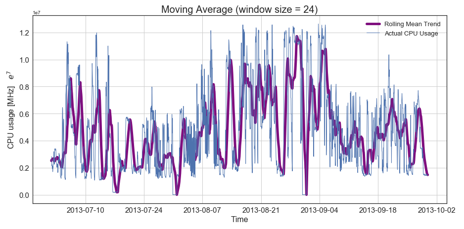
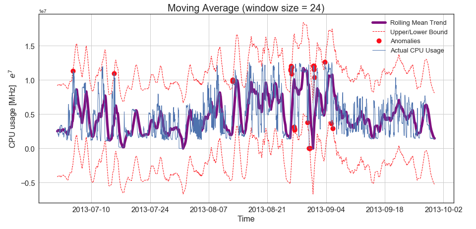
Figure 2. Moving averages in hourly data to capture higher level trends. Anomalies and confidence bounds shown red in second image (swipe to see).

Finally, I wanted to check the autocorrelations within the CPU Usage data in order to further assess the seasonality. In Figure 3. we can see again that CPU usage is a short-term time series (i.e., has short-term predictability), as evidenced by the high peaks early in the graph. Now that I have assessed some patterns in the data, I wanted to test a few models and see how well they were able to predict future CPU usage.

Figure 3. Autocorrelation plot for CPU usage.

Step 2. Exploratory Modeling

I tested a traditional linear regression model first. The model fit the data reasonably well, with a mean absolute percent error (MAE) of 34.19%. This very simple model’s predictions had the potential to reduce over-provisioning by a significant amount. However, there might be additional techniques that could help improve model accuracy. I also tried smoothing methods including a Holt-Winters model, which did not capture the seasonality of the data.

I then used a scaled linear regression model, again using time series train-test-split, and 5-fold-time-series-cross-validation. I also included time-lags ranging from 3–9 hours as additional features (I narrowed the range of time lags because of the short-term predictability of the data). This model fit the data slightly better (MAE = 31.14%). However, when looking at the predictive power of the coefficients, only the third time lag feature is significant. I also wanted to prevent overfitting. Therefore, next I tried feature reduction using regularization techniques including Lasso and Ridge regression. The scaled Ridge Regression model fit the data the best (MAE = 30.61%), compared to Lasso regression (MAE = 30.98%) and the previous models. I was successful in being able to model future CPU usage, as evidenced by an MAE of 30.61% for a highly variable dataset.

Figure 4. Scaled Ridge Regression Model (L2 regularization for feature reduction). MAE = 30.61%

Summary Part 1

I learned a great deal from initial exploration and early models. First, CPU usage is highly unpredictable and CPU usage is on average less than 7%. According to my models, a scaled Ridge Regression model made the most accurate predictions. L2 regularization found that the most significant predictors were previous time-lags. I also learned that the data has short-term predictability.

Part 2: Creating Real-Time Pipeline using a Recurrent Neural Network (RNN) on AWS

After initial exploration, I had a good sense of the data, but I needed to move towards a real-time pipeline for forecasting and prediction of CPU usage. This was an exciting new challenge.

Manifold wanted to be able to predict and forecast CPU usage 5–10 minutes in advance. In addition, the data contained 500 time series samples at a small time resolution. Finally, Manifold’s actual data is highly variable and dynamic. This necessitated that that I use a more sophisticated modeling approach.

To create a real-time prediction pipeline, I decided to move from using sklearn in Python to using DeepAR, a recently developed built-in deep learning algorithm in AWS Sagemaker, so I didn’t need to build my own model from scratch. DeepAR is a supervised learning algorithm for forecasting time series using a recurrent neural network (RNN). DeepAR works by training a single model jointly over a set of time series.

More details of my approach follow in the next sections.

Step 1: Develop Cleaning and Formatting Pipeline

Similar to Part 1, I started by pulling the activity data from 500 VMs over a three month time period into a pandas data frame using an EC2 instance on AWS. I converted the timestamp, which was in Unix epochs to a pandas date-time index. For this analysis, I used a finer time granularity (1-minute intervals). Next, I used a forward fill function to replace some missing values (DeepAR does not currently support missing or NA values). Finally, for cross-validation, I created the training data set from the testing data set by removing the prediction length (the last 30 minutes) from each time series.

DeepAR required the data be in JSON lines format, with each line representing a time series from one VM. To format the data accordingly, I indexed the pandas data frame by VM and date, created a list of with each time series, and finally converted them into JSON lines. I used a function to push all the formatted time series to an S3 bucket on AWS. Now that the data was cleaned, resampled, and correctly formatted, I could begin the modeling pipeline.

Step 2: Modeling Pipeline

To set up the modeling pipeline, first, I set initial hyperparameters based on observed characteristics of the data. I used a prediction and context length of 30 minutes (based on how far in advance I wanted to predict and also from how many minutes I wanted to base the predictions on). I used a two-layer RNN with 40 cells. I also used a learning rate of .001, a dropout rate of .05, and a student-t likelihood. I chose the student-t likelihood since it works well with “bursty”, or unpredictable data, like this dataset. Next, I trained the model using the training and testing data sets from my S3 bucket. After training the model, I used it to make predictions and deployed it to an endpoint in Sagemaker.

Figure 5. shows an example of the DeepAR model’s predictions for one time series (one VM). The model appears to be very accurate based on our visual exploration of the predictions. However, notice how my model (in orange) slightly underestimates the actual usage (the blue line). Therefore, in consultation with Manifold, I decided that they should take the upper bound of the forecast and add a cushion (e.g., 100 MHz) to reduce incidents of under-provisioning (shown in green). My Suggested Provision = Upper Limit + 100 CPU [MHz] cushion.

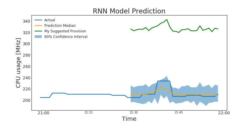
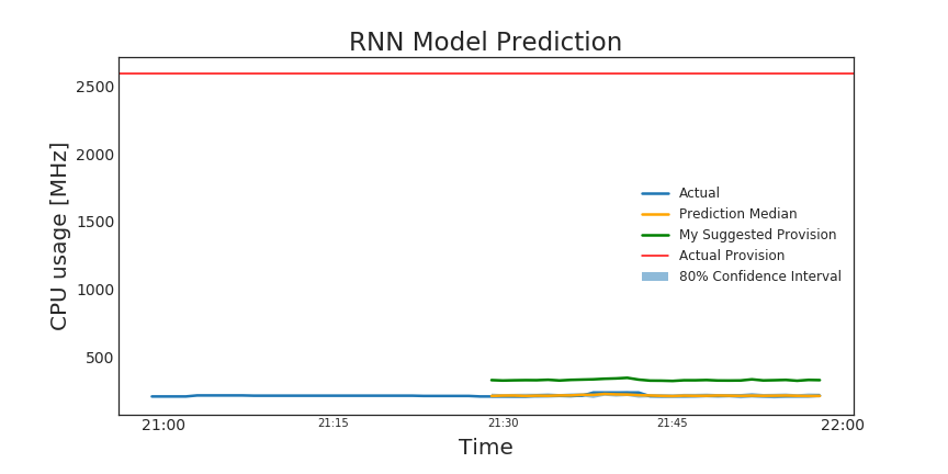
Figure 5. RNN model predictions (orange), my suggested provision (in green). While this might seem like my suggestion is high, in the context of what was originally provisioned (shown in red in second figure), we can see that my model significantly reduces over-provisioning and saves CPU.

Further, since Manifold will to optimize allocation in real-time, this means that failure to schedule resources based on prediction will not cause a failure in the system due to 1) redundant application copies running in the background, 2) fail-safes such as cushions (described above) applied in real-time, and 3) canary deployment. Canary deployment is a practice where you deploy a copy of new application, route a small portion of traffic to it (e.g., 10%), and test to see if it fails with the new configuration.

Step 3: Results

To quantify the actionable deliverable I made for Manifold, I randomly sampled two VM time series and calculated the CPU savings between my model’s CPU usage predictions and what CPU was actually provisioned for that VM.

Below in Figure 6. we can see that the original usage was only 23% of what was being provisioned. Compare this to my model, where my suggested limit, even with a large cushion, significantly reduces CPU over-provisioning, and now 82.3% of provisioned CPU is used.

Figure 6. Original usage ratio (left) compared to my model's usage ratio (right).

In a more dramatic example, for this VM time series, only 1.3% of CPU was being used compared to what was being provisioned. Compare this to my new model, which again greatly reduced over-provisioning.

Figure 7. Original usage ratio (left) compared to my model's usage ratio (right).

Summary of Part 2

With my model and real-time pipeline on AWS, I reduced projected CPU over-provisioning by up to 97% for a given VM time series, saving Manifold not only a great deal of time, but a great deal of money.

I also created a REST API where Manifold can route their usage data, apply my model, and then receive real-time predictions and forecasted usage for their applications. Manifold will implement this pipeline soon.

Finally, there is no added risk when applying my model to predict future usage, since neither the original provisions nor my suggested provisions under-provisioned.

Part 3: Actionable Deliverables